Note
Example data and Jupyter notebooks are included in the repository under the examples/ directory.
You can also follow along in the CCTA Notebook.
The stitching.py example script allows you to also display the trimesh debug plots.
Tutorial - CCTA Module
This step-by-step tutorial demonstrates how to:
Read in and label a CCTA geometry from an STL file and centerline CSV files
Prepare centerlines, detect branches, and discretize the vessel tree
Load an intravascular geometry and fine-align it to the CCTA point cloud
Label the anomalous (intramural) region within the CCTA mesh
Compute radial scaling factors for the proximal, distal, and aortic regions
Morph the CCTA mesh to match the intravascular geometry
Remove the intramural region and stitch the CCTA to the intravascular geometry
Remesh and smooth the stitched geometry
Visualise labeled regions and export section STL files
Re-label the final stitched geometry
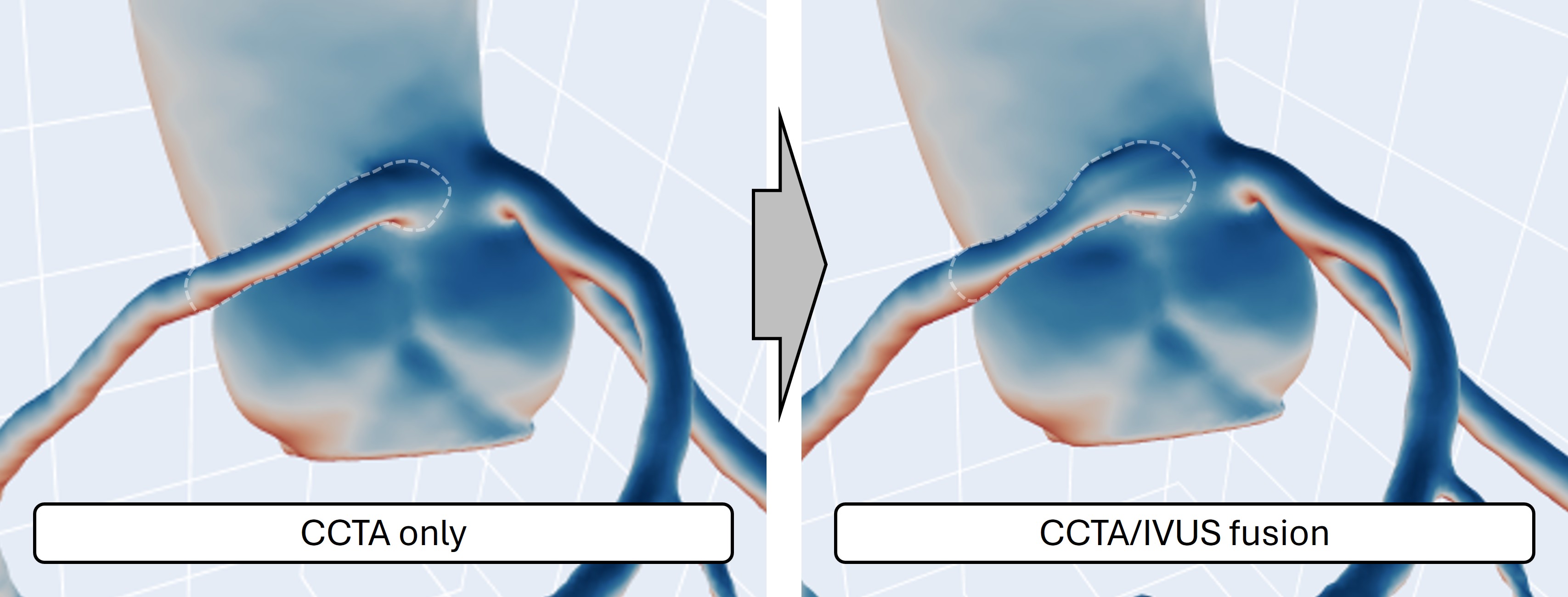
The goal of this module is to replace a section on the CCTA geometry with an intravascular geometry.
1. Read in and prepare CCTA geometries and centerlines
The entry point for the CCTA module is multimodars.label_geometry(), which reads a
triangulated surface mesh (STL) together with centerline CSV files for the aorta, the right
coronary artery (RCA), and the left coronary artery (LCA). It returns a labeled results
dictionary and three multimodars.PyCenterline objects that are used in all subsequent
steps.
import multimodars as mm

results, (rca_cl, lca_cl, ao_cl) = mm.label_geometry(
    path_ccta_geometry="data/NARCO_119_noside.stl",
    path_centerline_aorta="data/centerline_aorta.csv",
    path_centerline_rca="data/centerline_rca_short.csv",
    path_centerline_lca="data/centerline_lca.csv",
    bounding_sphere_radius_mm=3.0,
    n_points_intramural=100,
    anomalous_rca=True,
    anomalous_lca=False,
    control_plot=False,
)
Core algorithm labeling:
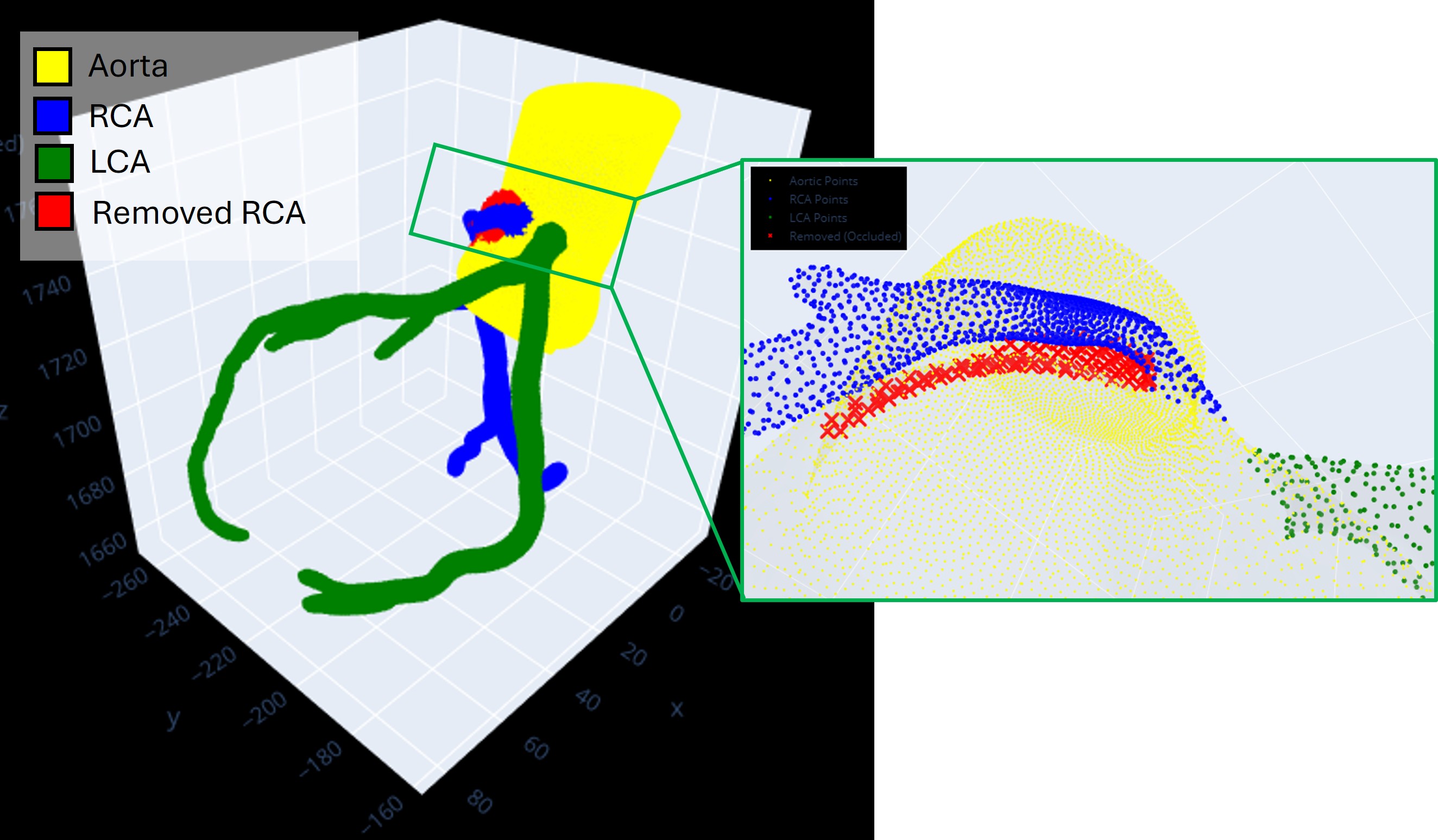
In the first step, a rolling sphere is propagated along the coronary centerlines. For anatomically normal coronary arteries, this approach reliably assigns all mesh vertices within the predefined radius to either the RCA or LCA label. In anomalous coronary arteries with an intramural course, however, the rolling sphere systematically mislabels a subset of aortic-wall vertices as coronary, owing to the compressed elliptic cross-section of the vessel and its proximity to the aortic wall (see Fig. 4).
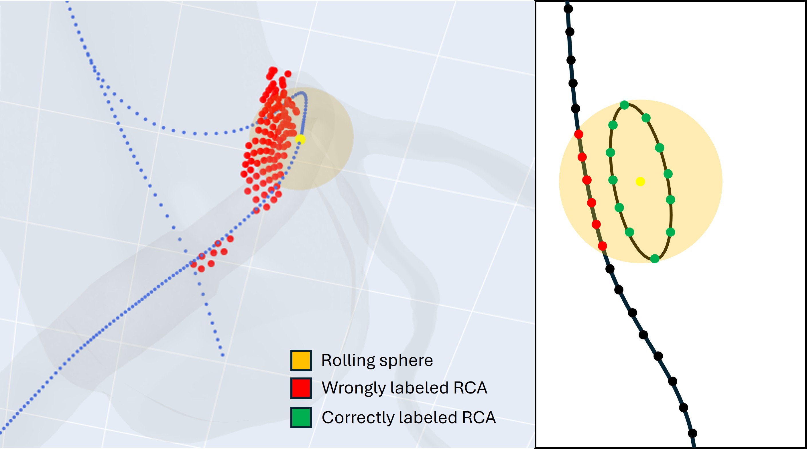
Fig. 4 Rolling sphere applied for the case of an R-AAOCA, demonstrating incorrect labeling caused by the elliptic vessel cross-section. Left: 3-D view; right: schematic illustration.
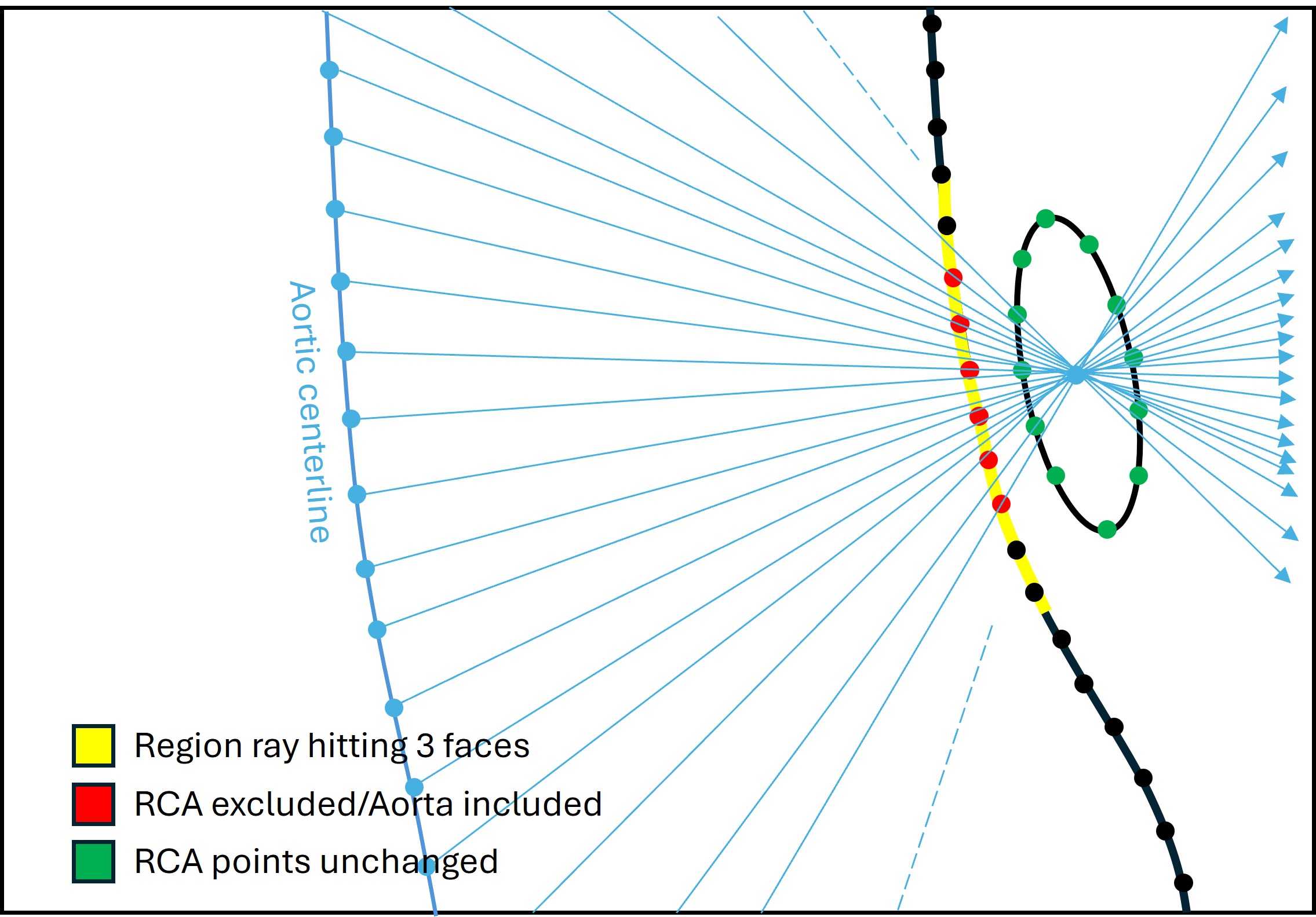
To address this limitation, a ray-casting algorithm is employed. A ray is cast from each aortic centerline point toward each of the n_points_intramural proximal coronary centerline points. When a ray intersects three mesh faces, the first intersected face is added to an occlusion set. All RCA vertices that are topologically connected to any face in this set are subsequently reclassified as aortic_points and recorded in rca_removed_points, removing them from the rca_points label. The identical procedure is applied symmetrically when anomalous_lca=True.
|
|
Left: 3D visualization of all cast rays. Right: schematic diagram of the occlusion-detection step.
As a final clean-up, any RCA or LCA vertex whose immediate mesh neighbours carry no
same-label assignment — an island vertex disconnected from all other coronary-labeled
vertices — is reclassified as aortic. This adjacency-based elimination ensures that
the returned rca_points and lca_points sets form topologically connected regions
on the mesh surface.
Parameter reference:
bounding_sphere_radius_mm: radius of the rolling sphere used for the initial vessel labeling pass. Larger values cast a wider net and capture more distant vertices; smaller values are more conservative. The default of 3.5 mm works for most datasets; adjust downward if neighboring structures are incorrectly captured.n_points_intramural: number of centerline points used to define the end of the intramural segment. When uncertain, keep this value large; the anomalous-region labeling in step 3 will refine the boundary.anomalous_rca/anomalous_lca: whenTrue, the algorithm removes incorrectly labeled intramural points from the respective vessel and reassigns them to"rca_removed_points"/"lca_removed_points". Set toFalsefor normal coronary anatomy.control_plot: opens an interactive 3-D scene to inspect the labeling result. Set toTruewhen tuningbounding_sphere_radius_mmorn_points_intramural.
The returned results dictionary contains:
"mesh"— the CCTA geometry as atrimesh.Trimeshobject."aorta_points"— vertices labeled as aorta:[(x, y, z), ...]."rca_points"— vertices labeled as RCA:[(x, y, z), ...]."lca_points"— vertices labeled as LCA:[(x, y, z), ...]."rca_removed_points"— RCA vertices inside the intramural course that were removed from the RCA label:[(x, y, z), ...]."lca_removed_points"— same for LCA.
The centerline CSV files must contain three columns (no header): x, y, z in mm.
They can be converted to multimodars.PyCenterline objects with normals using
multimodars.numpy_to_centerline():
import numpy as np

rca_cl_raw   = np.genfromtxt("data/centerline_rca_short.csv", delimiter=',')
lca_cl_raw   = np.genfromtxt("data/centerline_lca.csv",       delimiter=',')
aorta_cl_raw = np.genfromtxt("data/centerline_aorta.csv",     delimiter=',')

rca_cl   = mm.numpy_to_centerline(rca_cl_raw)
lca_cl   = mm.numpy_to_centerline(lca_cl_raw)
aorta_cl = mm.numpy_to_centerline(aorta_cl_raw)
2. Prepare centerlines, detect branches, and discretize the vessel tree
Before discretizing the vessel geometry, both coronary centerlines must have their branches
detected and the surface-mesh points labeled by branch. multimodars.prepare_centerlines()
handles all of this in a single call: it runs calculate_branches and check_centerline
on each centerline, then calls multimodars.label_branches() so the results dictionary
gains keys rca_points_main, rca_points_side_1, …, lca_points_main,
lca_points_side_1, …:
rca_cl, lca_cl, results = mm.prepare_centerlines(
    rca_cl, lca_cl, results,
    branch_sigma=2.0,
    control_plot=False,   # True opens a trimesh scene of the branch assignment
)
Parameter reference:
branch_sigma: Gaussian smoothing radius (mm) applied during branch detection. Increase if the algorithm over-segments a noisy centerline; decrease to preserve fine anatomical detail.control_plot: opens an interactive trimesh scene coloured by branch ID and showing the labelled surface points, so you can verify the assignment before discretizing.
Inspecting and correcting sharp angles
Noisy centerlines sometimes contain kinks that cause branch detection to misfire.
multimodars.find_sharp_angles() scans a branch for positions where the local tangent
reverses by more than the supplied cosine threshold and opens an optional debug scene with each
flagged position highlighted in a distinct colour:
# Inspect: red × marks every position that may need a correction
mm.plot_centerline_edges(lca_cl, cos_threshold=0.0)

# Find flagged positions (returns a list of 0-based indices within the branch)
positions = mm.find_sharp_angles(lca_cl, branch_id=0, cos_threshold=0.0,
                                 control_plot=True)
Once you know which positions need fixing, use split_branch to break a spurious loop and
merge_branches to re-attach the tail back onto the main vessel, then re-validate and
re-label. After splitting and merging it is assured that the longest centerline section will always be at position 0:
# Example: the 5th flagged position creates a loop — split there, then re-merge
lca_cl = lca_cl.split_branch(0, positions[4])
lca_cl = lca_cl.merge_branches(0, 4)
lca_cl = lca_cl.check_centerline()
results = mm.label_branches(lca_cl, results, results_key="lca_points")
Note
prepare_centerlines() cannot automate the split_branch /
merge_branches step because the right corrections are case-specific. Inspect the
control_plot output first, then call those methods manually before proceeding.
Discretizing the vessel tree
multimodars.discretize_vessel_tree() slices each vessel along its centerline at fixed
arc-length intervals and samples n_points evenly-spaced points from each cross-sectional
contour. It also computes an orientation reference triplet (main, counter-clockwise, and
clockwise reference points) at the ostium and at every side-branch bifurcation. These
triplets are stored in tree.rca_references and tree.lca_references and are later
used to initialize the three-point alignment in step 3:
tree = mm.discretize_vessel_tree(
    ao_cl, rca_cl, lca_cl,
    results,
    step_size=1.0,      # arc-length spacing between cross-sections in mm
    n_points=100,       # points per output contour ring
    b_spline=True,      # replace each contour with a closed B-spline fit
    bspline_smoothing=5.0,
    control_plot=False, # True opens a trimesh scene of the full tree
)

# Inspect the result interactively
mm.plot_vessel_tree(tree)
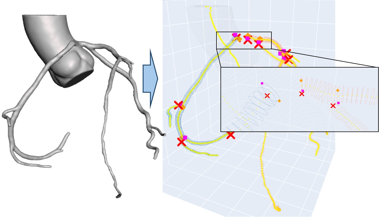
Fig. 5 The original 3-D model of the CCTA is discretized with a predefined step size (here 1 mm). This allows to easily detected reference points, and additionally perform measurements for different positions, since all slices are stored as PyContours.
Parameter reference:
step_size: arc-length distance between consecutive cross-sections in mm. Smaller values give finer sampling but increase memory use.n_points: number of evenly-spaced points per output contour ring. 100 is a good default; reduce to 50 for a lightweight preview.b_spline: whenTrue, each discretized contour is replaced with a closed periodic B-spline fit before the reference points are computed. Useful when raw contours are noisy.bspline_smoothing: smoothing conditionsforsplprep.0= exact interpolation;≈ n_points= gentle smoothing;≈ 5 x n_points= strong smoothing. Tune empirically based on how irregular the raw contours appear.bspline_degree: B-spline polynomial degree (default 3, cubic).
The discretized tree exposes the following attributes:
tree.discretized_aorta— list ofPyContourfor the aorta.tree.discretized_rca_main/tree.discretized_lca_main— main-vessel contours.tree.rca_branches/tree.lca_branches— list of lists, one per side branch.tree.rca_references/tree.lca_references— list of(main_ref, ccw_ref, cw_ref)triplets, one per bifurcation site.
3. Load and align intravascular geometry
Load the intravascular segmentation with multimodars.from_file_singlepair() (see the
Tutorial - Intravascular Module for the full range of loading options and parameter tuning):
rest, (dia_logs, sys_logs) = mm.from_file_singlepair(
    input_path="ivus_rest",
    labels=["aligned_dia", "aligned_sys"],
    output_path="output/rest",
)
Once the intravascular geometry is loaded, align it to the CCTA centerline and point cloud
with multimodars.align_combined(). This function first performs a coarse three-point
alignment using the reference triplet computed in step 2, and then refines the rotation by
minimising Hausdorff distances between the CCTA point cloud and the intravascular contours.
The reference triplet (main_ref_pt, counterclockwise_ref_pt, clockwise_ref_pt) at the
RCA ostium is available directly from the discretized tree:
ref_points = tree.rca_references[0]   # triplet at the ostium (index 0)
rca_cl_main = rca_cl.get_branch(0)    # alignment needs a single-branch centerline

aligned, resampled_cl = mm.align_combined(
    rca_cl_main,
    rest,
    ref_points[0],                     # main reference point
    ref_points[1],                     # counter-clockwise reference point
    ref_points[2],                     # clockwise reference point
    results['rca_points'],             # CCTA point cloud for Hausdorff refinement
    angle_range_deg=10.0,
    write=True,
    watertight=False,
    output_dir="test",
)
Parameter reference:
angle_range_deg: angular search window (±degrees) for the Hausdorff refinement step around the initial three-point estimate. Reduce to speed up computation once the approximate orientation is known.write/watertight/output_dir: whenwrite=True, OBJ meshes are exported tooutput_dir;watertight=Truecloses the ends with cap vertices.
4. Label the anomalous region
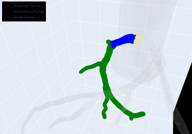
After alignment, multimodars.label_anomalous_region() subdivides the RCA points into
three sub-regions — proximal, anomalous (intramural), and distal — based on the spatial
overlap between the aligned intravascular frames and the CCTA mesh:
results = mm.label_anomalous_region(
    centerline=rca_cl,
    frames=aligned.geom_a.frames,
    results=results,
    results_key='rca_points',
    debug_plot=False,
)
The results dictionary is extended with:
"proximal_points"— RCA vertices proximal to the anomalous segment."anomalous_points"— RCA vertices inside the intramural segment."distal_points"— RCA vertices distal to the anomalous segment.
Set debug_plot=True to open an interactive scene that shows how the three sub-regions
are assigned — useful when the boundary appears misplaced.
5. Compute scaling factors
Before morphing the mesh, the optimal scaling factor for each region must be computed. Each function searches for the radial scale that minimises the distance between the CCTA mesh and the corresponding portion of the aligned intravascular geometry.
Proximal and distal scaling
multimodars.find_distal_and_proximal_scaling() finds the best radial scale for the
first and last frames of the intravascular geometry relative to the proximal and distal CCTA
vertices respectively:
prox_scaling, distal_scaling = mm.find_distal_and_proximal_scaling(
    frames=aligned.geom_a.frames,
    centerline=rca_cl,
    results=results,
)
Both return values are signed floats in mm: positive means the CCTA vertex ring is expanded, negative means it is contracted, relative to the intravascular contour.
Aortic scaling
multimodars.find_aorta_scaling() optimizes the radial scale of the aortic region by
minimising the distance between the aortic CCTA vertices and the outer wall of the anomalous
intravascular geometry:
aortic_scaling = mm.find_aorta_scaling(
    frames=aligned.geom_a.frames,
    cl_aorta=ao_cl,
    results=results,
)
Aortic wall scaling
For anomalous coronary arteries, an additional scaling factor targets the aortic wall
vertices ("rca_removed_points" region) and aligns them with the first intravascular
frame whose lumen elliptic ratio drops below 1.3 — the transition from compressed intramural
to round free-segment lumen:
aortic_wall_scaling = mm.find_aortic_wall_scaling(
    frames=aligned.geom_a.frames,
    cl_aorta=ao_cl,
    results=results,
)
Note
find_aortic_wall_scaling raises ValueError if no frame with elliptic ratio < 1.3
is found. This can happen when the intramural segment is very short or the geometry is
nearly circular throughout. In that case, omit this scaling step.
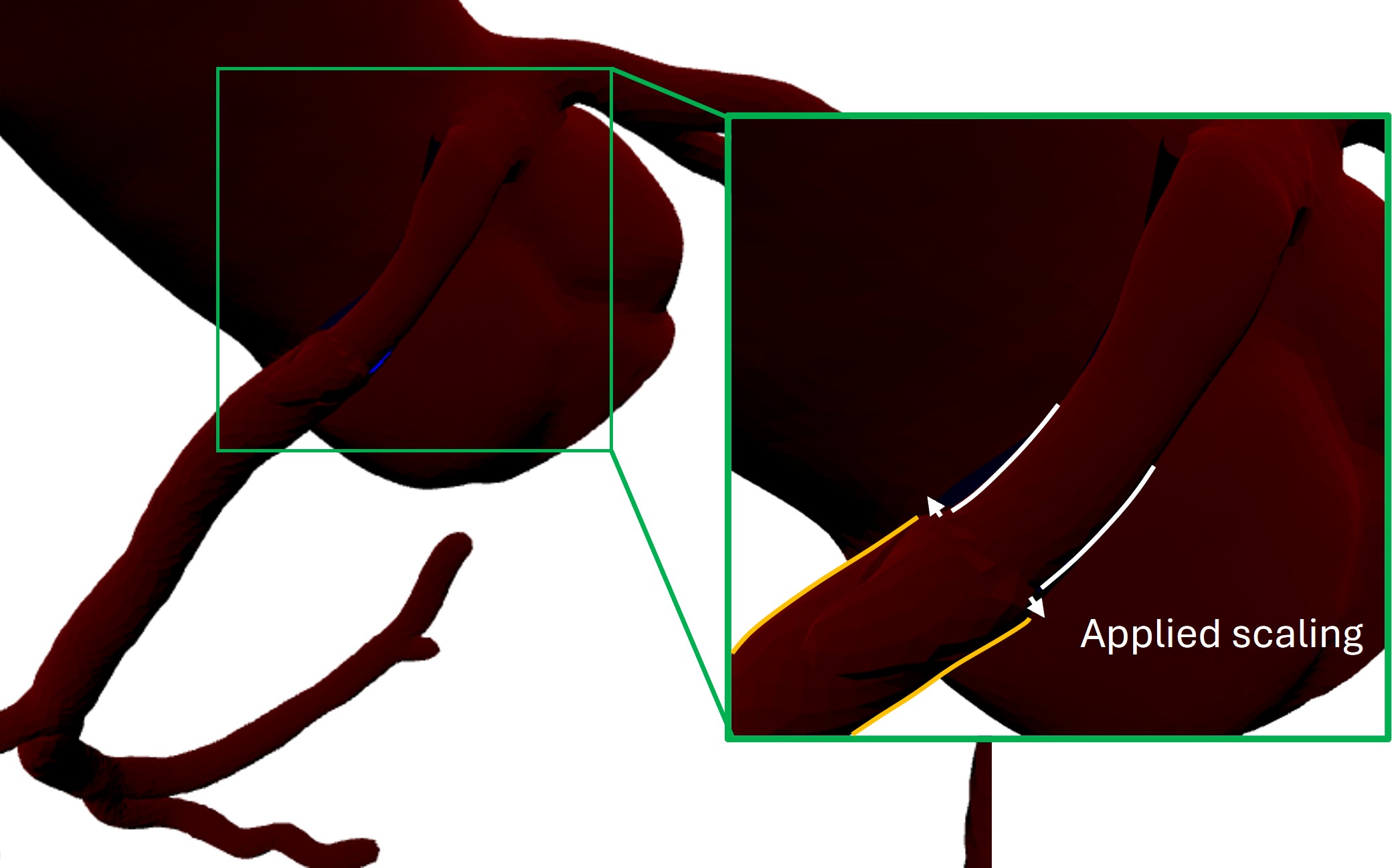
Here the created wall in the alignment module (based of measurement_1 in record data from PyInputData)
is used to minimize distance between the intravascular wall and the removed_rca_points on the ccta mesh (see Fig. 6).
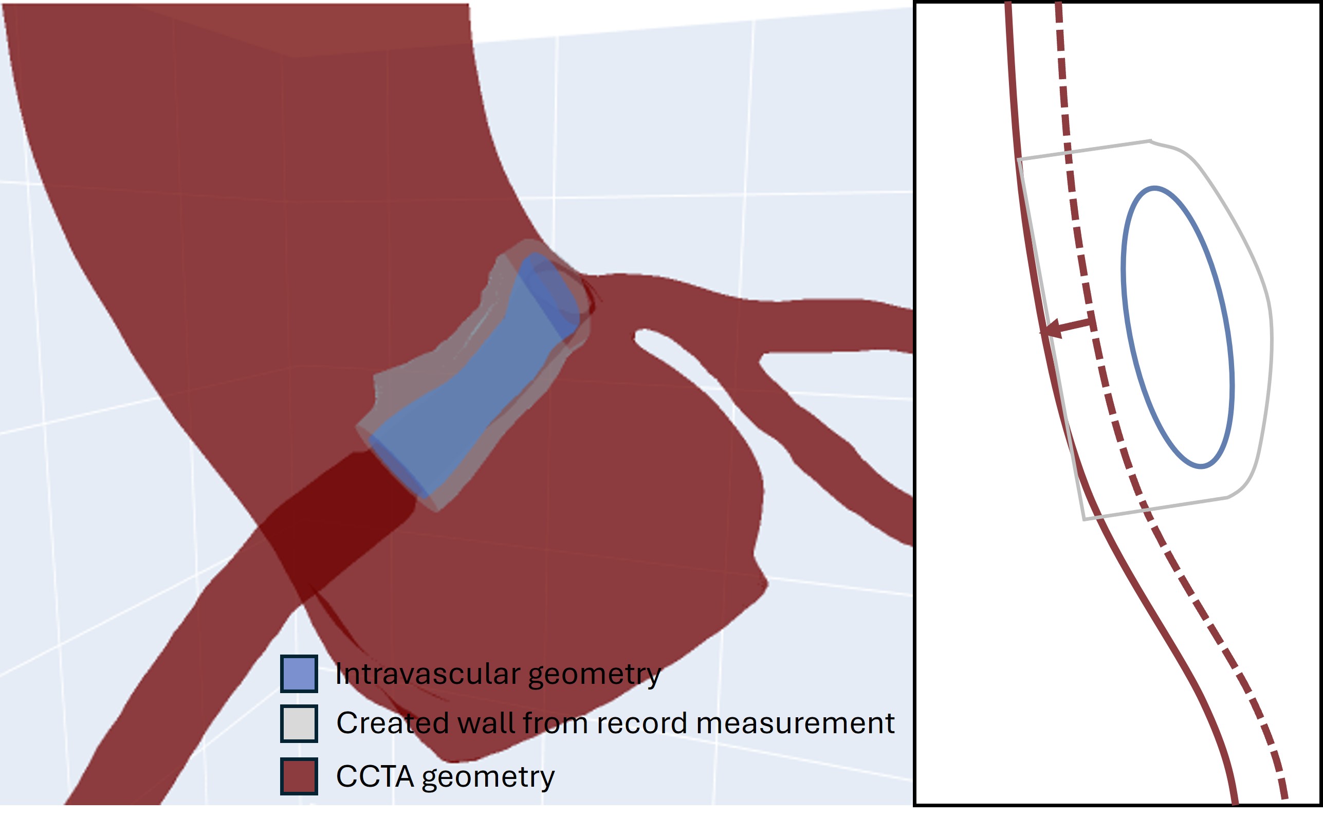
Fig. 6 R-AAOCA with aligned intravascular mesh, scaled distal coronary and scaled aorta to match the Wall in PyGeometry. Left: 3-D view; right: schematic illustration.
6. Morph CCTA to intravascular geometry
Each region is morphed independently with multimodars.scale_region_centerline_morphing().
The function moves mesh vertices radially along the local centerline normal so that the
region diameter changes by diameter_adjustment_mm. Because the mesh is modified in
place, multimodars.sync_results_to_mesh() must be called after each morphing step to
keep the coordinate lists in results consistent with the updated vertex positions:
# 1. Scale the distal segment
scaled_distal = mm.scale_region_centerline_morphing(
    mesh=results['mesh'],
    region_points=results['distal_points'],
    centerline=rca_cl,
    diameter_adjustment_mm=distal_scaling,
)
results = mm.sync_results_to_mesh(results, results['mesh'], scaled_distal)

# 2. Scale the aortic region (aorta + intramural wall) along the aortic centerline
scaled_aortic = mm.scale_region_centerline_morphing(
    mesh=results['mesh'],
    region_points=results['aorta_points'] + results['rca_removed_points'],
    centerline=aorta_cl,
    diameter_adjustment_mm=aortic_scaling,
)
results = mm.sync_results_to_mesh(results, results['mesh'], scaled_aortic)

# 3. Scale the proximal segment
scaled_proximal = mm.scale_region_centerline_morphing(
    mesh=results['mesh'],
    region_points=results['proximal_points'],
    centerline=rca_cl,
    diameter_adjustment_mm=prox_scaling,
)
results = mm.sync_results_to_mesh(results, results['mesh'], scaled_proximal)
Note
The order of morphing steps matters because each call to
sync_results_to_mesh() updates all point lists to reflect the current
mesh state. Always sync before passing results['mesh'] to the next morphing call.
7. Remove intramural region and stitch geometries
Before stitching, remove the anomalous and proximal regions from the CCTA mesh. This opens
a boundary ring at the proximal end of the intravascular segment where the two meshes will
be connected. multimodars.remove_labeled_points_from_mesh() deletes the requested
vertices, remaps the remaining faces, and adds a "boundary_points" key to results:
updated_results = mm.remove_labeled_points_from_mesh(
    results,
    ["anomalous_points", "proximal_points"],
)
region_keys accepts a single string or a list of strings matching keys in results.
Any combination of labeled regions can be removed; the resulting open boundary is always
placed adjacent to the deleted vertices.
Once the hole is open, multimodars.stitch_ccta_to_intravascular() connects the
boundary ring of the CCTA mesh to the proximal contour of the aligned intravascular
geometry with a triangulated patch:
stitched = mm.stitch_ccta_to_intravascular(
    aligned.geom_a,
    updated_results['mesh'],
    updated_results,
    prox_start_mode="highest_z",
)
Parameter reference:
n_points_iv_cont: number of points to which each intravascular contour is downsampled before stitching (default 100). Matching this to the boundary-ring resolution improves triangle quality.prox_start_mode/dist_start_mode: controls which vertex is chosen as index 0 of the boundary ring before the rings are paired for stitching."nearest_iv"(default) — rotate to the boundary vertex closest to intravascular point 0. Works well when the two point sets share a consistent anatomical orientation."highest_z"— rotate to the boundary vertex with the largest z-coordinate. Prefer this when the pullback axis is nearly aligned with the image z-axis, as is common for straight intramural segments.
clamp_overshoot: minimum distance in mm that every proximal boundary point must sit away from the IV plane after clamping (default 0.5). Only active for anomalous ostia where the boundary-ring plane and the IV plane diverge by ≥ 45°. Increase this value if stitching artefacts remain visible near the ostium; decrease it (toward 0.0) for more tightly fitted geometries.
The return value is a new results-like dictionary that additionally contains:
"prox_boundary_points"— the ordered proximal boundary ring used for stitching."dist_boundary_points"— the ordered distal boundary ring.
Export the raw stitched mesh before remeshing to allow inspection:
stitched['mesh'].export("prefixed_mesh.stl")
8. Remesh and smooth
The stitched mesh typically contains boundary artefacts and irregular triangulation where
the two surfaces meet. multimodars.fix_and_remesh_stitched_mesh() applies a three-step
repair and remeshing pipeline (non-manifold repair → hole filling → isotropic remesh) using
pymeshlab:
import trimesh

remeshed = stitched.copy()
remeshed['mesh'] = mm.fix_and_remesh_stitched_mesh(
    stitched['mesh'],
    target_edge_length_mm=0.5,
    verbose=True,
)
print(f"Watertight? {remeshed['mesh'].is_watertight}")
Note
fix_and_remesh_stitched_mesh requires the optional pymeshlab dependency.
Install it with pip install 'multimodars[meshlab]'.
Parameter reference:
target_edge_length_mm: desired edge length after isotropic remeshing. IfNone, uses the 25th-percentile edge length of the input mesh (preserves the fine intravascular mesh resolution as the reference).remesh_iterations: number of isotropic remeshing iterations (default 10). More iterations improve regularity at the cost of computation time.verbose: print per-step vertex/face counts and watertightness.
After remeshing, apply Taubin smoothing to reduce surface noise while preserving overall shape:
trimesh.smoothing.filter_taubin(remeshed['mesh'], lamb=0.6)
remeshed['mesh'].export("fixed_mesh.stl")
9. Visualise and export sections
Inspect the labeled regions of the stitched result with multimodars.plot_results_key().
Pass True for each region you want to highlight:
mm.plot_results_key(stitched)                   # aorta_points only (default)
mm.plot_results_key(stitched, False, True)      # rca_points only
Colour coding:
Yellow — aortic points
Blue — RCA coronary points
Green — LCA coronary points
Red — removed / intramural points
Cyan — proximal points
Magenta — distal points
Orange — anomalous points
To inspect the stitching seam directly, overlay the proximal boundary ring with the intravascular contour in a trimesh scene. The following snippet colours the boundary ring from red (index 0) to blue (last index) and overlays the frame-0 lumen points of the downsampled intravascular geometry:
import numpy as np
import trimesh

boundary_pts = np.array(remeshed['prox_boundary_points'], dtype=np.float64)
sphere_meshes = []
for i, pt in enumerate(boundary_pts):
    t = i / max(len(boundary_pts) - 1, 1)
    color = [int(255 * t), 0, int(255 * (1 - t)), 200]
    s = trimesh.creation.icosphere(radius=0.1).apply_translation(pt)
    s.visual.face_colors = color
    sphere_meshes.append(s)

iv_viz = aligned.geom_a.downsample(100).sort_frame_points()
iv_pts = iv_viz.frames[0].lumen.points
n_iv = len(iv_pts)
for pt in iv_pts:
    t = pt.point_index / max(n_iv - 1, 1)
    color = [int(255 * t), 0, int(255 * (1 - t)), 220]
    s = trimesh.creation.icosphere(radius=0.15).apply_translation([pt.x, pt.y, pt.z])
    s.visual.face_colors = color
    sphere_meshes.append(s)

spheres = trimesh.util.concatenate(sphere_meshes)
scene = trimesh.Scene([remeshed['mesh'], spheres])
scene.show()
Export individual anatomical sections as STL files with multimodars.export_section_stl().
The type argument controls which region is exported:
mm.export_section_stl(stitched, "all")    # full mesh
mm.export_section_stl(stitched, "aorta")  # aorta + intramural wall
mm.export_section_stl(stitched, "rca")    # RCA segment with adjacent aortic ring
mm.export_section_stl(stitched, "lca")    # LCA segment with adjacent aortic ring
An optional output_dir argument specifies the destination folder (defaults to the current
working directory). The exported filenames are all.stl, aorta.stl, rca.stl, and
lca.stl respectively.
To extract a sub-mesh programmatically (e.g. to pass to a downstream analysis), use
multimodars.keep_labeled_points_from_mesh():
aorta_mesh = mm.keep_labeled_points_from_mesh(stitched, "aorta_points")
10. Re-label the final geometry
After remeshing and smoothing, the vertex coordinates have changed and the stored point
lists are no longer valid. Re-running multimodars.label_geometry() on the exported
fixed mesh produces a fresh, consistent labeling that can be used for downstream
biomechanical simulation or further analysis:
results, (rca_cl, lca_cl, ao_cl) = mm.label_geometry(
    path_ccta_geometry="fixed_mesh.stl",
    path_centerline_aorta="data/centerline_aorta.csv",
    path_centerline_rca="data/centerline_rca_short.csv",
    path_centerline_lca="data/centerline_lca.csv",
    bounding_sphere_radius_mm=3.0,
    n_points_intramural=100,
    anomalous_rca=True,
    anomalous_lca=False,
    control_plot=True,
)

mm.export_section_stl(results, "all")
mm.export_section_stl(results, "aorta")
mm.export_section_stl(results, "lca")
mm.export_section_stl(results, "rca")