Note

Example data and Jupyter notebooks are included in the repository under the examples/ directory. You can also follow along in the Intravascular Notebook.

Tutorial - Intravascular Module

This step-by-step tutorial demonstrates how to:

1. Prepare segmentation data for best results

2. Run the workflow from CSV files (AIVUS-CAA output)

3. Run the workflow from numpy arrays — including in-depth parameter finetuning

4. Align a geometry with a CCTA centerline

5. Save geometries as .obj files

6. Convert between Py* objects and numpy arrays

7. Use class-level methods for inspection and manipulation

1. General note on segmentation preparation

The package is designed to work with segmented intravascular images from either IVUS or OCT. Segmentation must, however, follow specific conventions to ensure optimal results. The package was developed with coronary artery anomalies in mind, and specifically anomalous aortic origin of a coronary artery (AAOCA) with an intramural course, in which part of the vessel traverses the aortic wall. In all cases, it is essential to define a correct anatomical reference point to enable subsequent co-registration with the CCTA geometry (see Fig. 1).

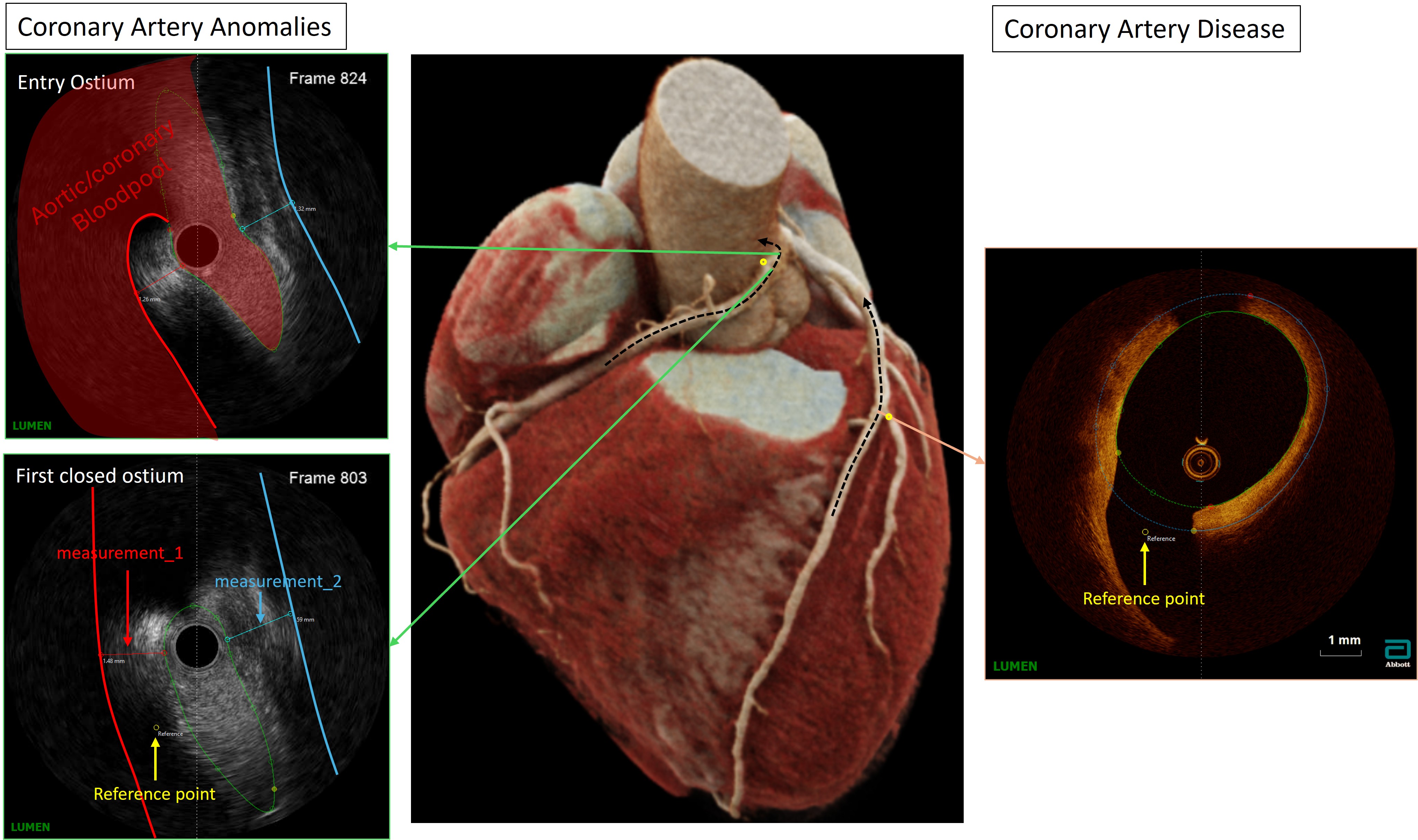
Fig. 1 Reference point placement for intravascular segmentation data preparation.

For coronary artery disease (CAD), it is sufficient to identify a bifurcation and place the reference point at the ostium of the side branch. For AAOCA, it is important to first identify the most proximal fully closed lumen contour in both diastole and systole, and subsequently place the reference point at the centre of the vessel on the aortic side (see also True pulsatile lumen visualization in coronary artery anomalies using controlled transducer pullback and automated IVUS segmentation).

Rationale for the four processing modes. The four alignment modes — full, double-pair, single-pair, and single — reflect the number of distinct geometric states that a given clinical question requires. In a standard controlled-speed IVUS pullback, each anatomical position along the vessel is sampled repeatedly across cardiac cycles. When pullbacks are acquired under both rest and stress conditions, each position is represented by four independent geometric states: rest-diastole, rest-systole, stress-diastole, and stress-systole. This is particularly relevant in AAOCA, where the intramural segment undergoes a complex, phase- and load-dependent deformation that can only be fully characterised by comparing all four states simultaneously (full mode).

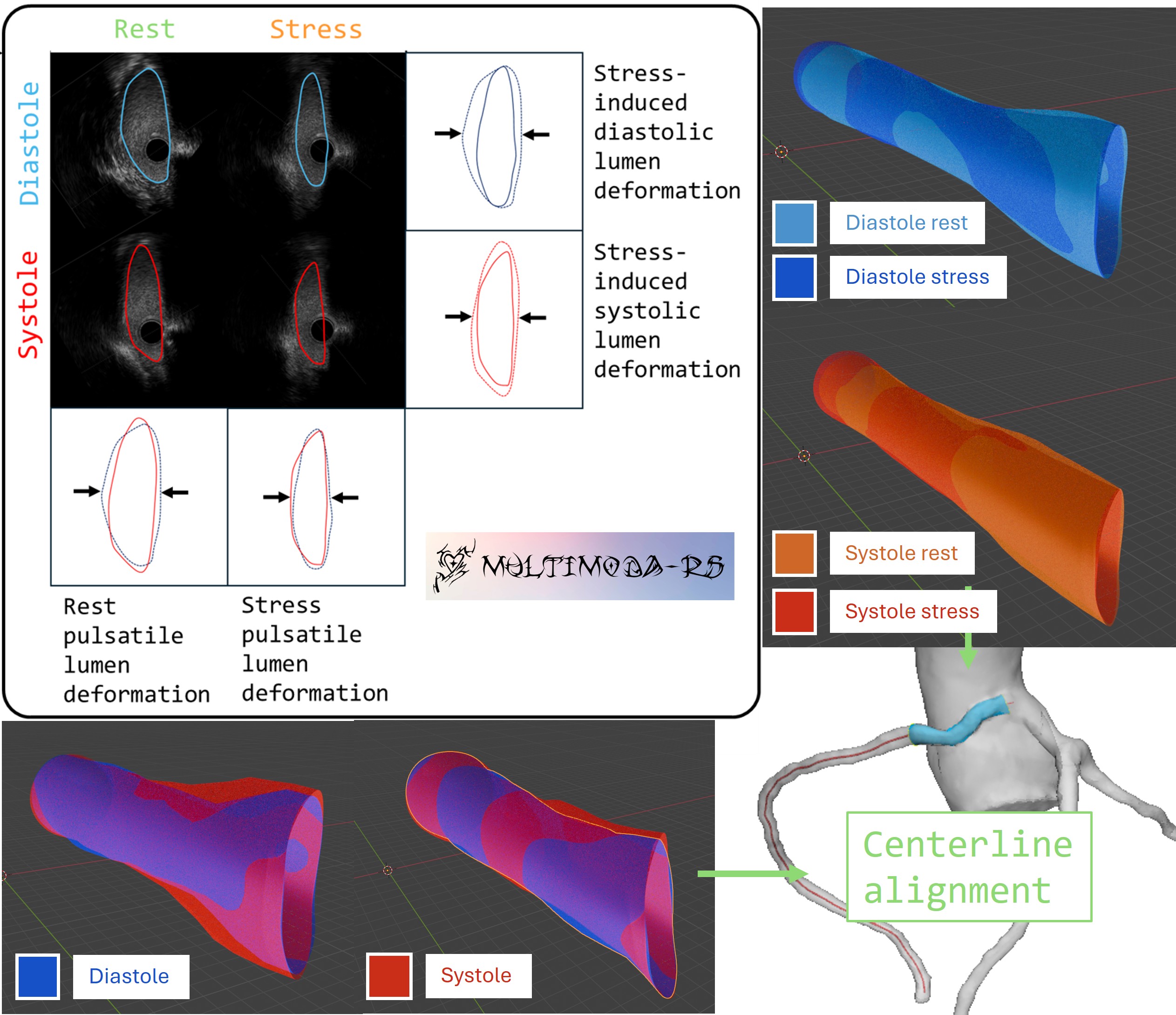
Fig. 2 Overview of the four processing modes supported by the package.

An important practical consequence is that heart rate differs between rest and stress. Because the catheter is withdrawn at a constant speed, a higher heart rate during stress results in a greater number of cardiac cycles — and thus a greater number of diastolic-systolic pairs — per unit of pullback length. Consequently, the axial inter-frame spacing is effectively compressed at stress relative to rest, and the two pullbacks must be resampled to a common z-grid before any cross-condition comparison can be made. The alignment algorithms in this package account for this discrepancy automatically.

Although the full mode was designed with AAOCA in mind, all four modes are directly applicable to other clinical contexts. In coronary artery disease, for example, single-pair mode is well suited to comparing diastolic and systolic frames within a single pullback, while single mode supports standalone geometry reconstruction for pre- or post-intervention assessment. The double-pair mode is appropriate whenever two independent pullbacks must be compared (e.g., pre- vs. post-stenting, or two different patients) without the additional stress-rest dimension.

2. Workflow csv files

Note

This workflow is based on the output of the AIVUS software. The preferred workflow for a more general workflow is to directly use numpy arrays, which can be easily created from the csv files, but also from any other source. The csv workflow is provided for users who are already using AIVUS and want to quickly apply the package to their data.

After pip installing or locally building the package, install it in the familiar way.

import multimodars as mm

To run the whole workflow from .csv files with either multimodars.from_file_full(), multimodars.from_file_doublepair(), multimodars.from_file_singlepair() or multimodars.from_file_single() the following requirements have to be met. Files should be named after AIVUS convention: diastolic_contours.csv, systolic_contours.csv, diastolic_reference_points.csv and systolic_reference_points.csv depending on the required analysis. Every file should be structured in the following way (the files themselves have no headers):

frame_index	x (mm)	y (mm)	z (mm)
…	…	…	…
771	2.4862	6.7096	24.5370
771	2.5118	6.7017	24.5370
771	2.5370	6.6936	24.5370
…	…	…	…

Column descriptions:

• frame_index — integer identifier of the imaging frame along the pullback sequence. All contour points that belong to the same cross-sectional slice share the same index. Frames do not need to be contiguous or start at zero; the package groups rows by this value.

• x, y, z — 3D Cartesian coordinates of the contour point in millimetres (mm). The coordinate system is that of the segmentation software (typically the image plane x/y plus the pullback depth z). Providing pixel values instead of physical coordinates will produce incorrect area and distance measurements downstream.

Optionally a record file can be provided combined_sorted_manual.csv, which should have the following structure, here the first column should contain the desired frame order and “measurement_1” represent the thickness of the wall between aorta and coronary and “measurement_2” for the thickness between pulmonary artery and coronary (position just for demonstration) (see Fig. 1). This is based on the output of the AIVUS-CAA software:

frame	(position)	phase	measurement_1	measurement_2
18	23.99	D
37	22.79	D		2.35
212	21.59	D	1.38	2.34
94	20.39	D	1.38	2.11
…	…	…	…	…
47	18.78	S

The full workflow comparing rest vs. stress and diastole vs. systole can be run with multimodars.from_file_full():

rest, stress, dia, sys, _ = mm.from_file_full(
    input_path_ab="ivus_rest",
    input_path_cd="ivus_stress",
    step_rotation_deg=0.1,
    range_rotation_deg=90,
    image_center=(4.5, 4.5),
    radius=0.5,
    n_points=20,
    write_obj=True,
    watertight=False,
    contour_types=[mm.PyContourType.Lumen, mm.PyContourType.Catheter, mm.PyContourType.Wall],
    output_path_ab="output/rest",
    output_path_cd="output/stress",
    output_path_ac="output/diastole",
    output_path_bd="output/systole",
    interpolation_steps=28,
)

The workflow can also be simplified by leaving the default values and only providing input and output paths, here e.g. for a singlepair:

rest, (dia_logs, sys_logs) = mm.from_file_singlepair(
    input_path="ivus_rest",
    output_path="output/rest",
)

3. Workflow numpy arrays

Note

CSV vs. numpy workflow — The CSV workflow (section 2) reads contour files directly from disk and is the fastest path when your data already comes from AIVUS-CAA. The numpy workflow accepts data from any source: you build multimodars.PyInputData objects manually and then call the same alignment functions. Choose the numpy workflow when your segmentation software uses different file formats, when you want to apply pre-processing steps (filtering, resampling, coordinate transforms) before alignment, or when you are embedding multimodars into a larger pipeline. Both workflows call identical underlying algorithms; only the input preparation differs.

To call multimodars.from_array_full(), multimodars.from_array_doublepair(), multimodars.from_array_singlepair() or multimodars.from_array_single() the contours and reference point must be packed into a multimodars.PyInputData object first using multimodars.numpy_to_inputdata(). We assume that before_arr, after_arr, before_ref and after_ref are all numpy arrays of shape (N, 4) (same column order as the CSV files: frame index, x in mm, y in mm, z in mm):

before_input_data = mm.numpy_to_inputdata(
    lumen_arr=before_arr,
    ref_point=before_ref,
    record=None,
    diastole=True,
    label="prestent",
)

after_input_data = mm.numpy_to_inputdata(
    lumen_arr=after_arr,
    ref_point=after_ref,
    record=None,
    diastole=True,
    label="poststent",
)

pair, _ = mm.from_array_singlepair(
    input_data_a=before_input_data,
    input_data_b=after_input_data,
    label="singlepair",
    output_path="output/stent_comparison",
    step_rotation_deg=0.01,
    range_rotation_deg=30,
)

Finetuning of alignment algorithms (in-depth parameter explanation)

The alignment algorithm co-registers adjacent intravascular frames by translating each frame to a common centroid and subsequently identifying the optimal rotation angle that minimises the Hausdorff distance between consecutive contours. Computational efficiency is achieved through a hierarchical coarse-to-fine angular search combined with multi-threaded processing of the different geometric states (see Fig. 3).

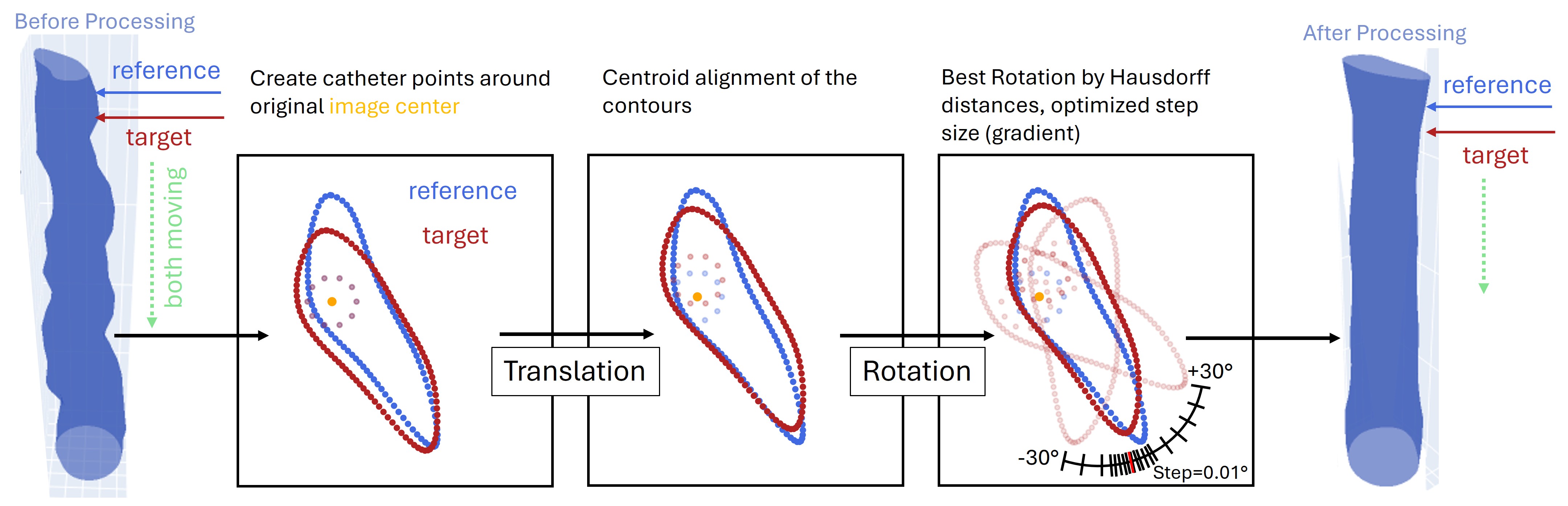
Fig. 3 Schematic of the translation and rotation alignment algorithm, illustrating the rotation search range, step size, image centre, and catheter radius parameters.

This section provides an in-depth discussion of each parameter, using multimodars.from_array_full() as a reference. The only required inputs are the four multimodars.PyInputData` objects (input_data_a through input_data_d); all remaining parameters have sensible defaults.

import multimodars as mm

rest, stress, diastole, systole, (log_rest, log_stress, log_diastole, log_systole) = mm.from_array_full(
    input_data_a=diastole_rest_input,    # REST diastole
    input_data_b=systole_rest_input,     # REST systole
    input_data_c=diastole_stress_input,  # STRESS diastole
    input_data_d=systole_stress_input,   # STRESS systole
    step_rotation_deg=0.5,
    range_rotation_deg=90,
    sample_size=500,
    image_center=(4.5, 4.5),
    radius=0.5,
    n_points=20,
    write_obj=True,
    watertight=True,
    contour_types=[mm.PyContourType.Lumen, mm.PyContourType.Catheter, mm.PyContourType.Wall],
    output_path_ab="output/rest_results",
    output_path_cd="output/stress_results",
    output_path_ac="output/diastole_results",
    output_path_bd="output/systole_results",
    interpolation_steps=0,
    bruteforce=False,
    smooth=True,
    postprocessing=True,
)

Parameter reference:

• step_rotation_deg and range_rotation_deg: define the angular search space and its resolution. The algorithm tests candidate rotations from -range_rotation_deg to +range_rotation_deg in increments of step_rotation_deg. In the example above, the full range of ±90° is explored at 0.5° resolution. When the approximate orientation is already known, reducing range_rotation_deg (e.g. to 30°) substantially reduces computation time without sacrificing accuracy.

• sample_size: contours are downsampled to at most this many points prior to Hausdorff distance computation. Contours with fewer points are left unchanged. The default of 500 points is appropriate for most IVUS datasets; increasing this value improves accuracy at the cost of computation time.

• image_center, radius, and n_points: these three parameters define the synthetic catheter used as an additional rotational anchor (see Fig. 3). image_center specifies the catheter centre as (x, y) in mm, radius the catheter radius in mm, and n_points the number of points sampled on the catheter circle.

Note

n_points controls the relative weight of the catheter position versus the lumen contour shape during alignment. A larger value makes the catheter centroid more influential, which benefits round, featureless contours where Hausdorff distances alone are ambiguous across different rotation angles. For geometrically distinct contours (e.g. severely stenotic or anomalous segments), a small value or even n_points=0 is more appropriate.

• write_obj and watertight: when write_obj=True, triangle meshes are constructed from the aligned contour points and exported as Wavefront OBJ files, together with a material file (.mtl) and a UV map encoding the per-vertex deformation relative to geometry A. Setting watertight=True closes the proximal and distal ends of each mesh by connecting the boundary contour points to a central cap vertex.

• contour_types: specifies which contour layers are exported. Three types are supported: Lumen (the vessel lumen boundary), Catheter (the synthetic catheter circle defined by image_center, radius, and n_points), and Wall (the aortic wall representation). The wall is derived from measurement_1 in the record file when provided; otherwise a uniform 1 mm outward offset is applied.

• output_path_ab, output_path_cd, output_path_ac, and output_path_bd: output directories for the four cross-aligned geometry pairs. The mapping between input slots and output paths is:

                   output_path_ac (Diastole: a vs. c)
         ┌──────────────────────────────────────────┐
         ▼                                          ▼
a REST diastole                      c STRESS diastole
      │  output_path_ab (Rest: a+b)        │  output_path_cd (Stress: c+d)
      ▼                                        ▼
b REST systole                       d STRESS systole
         └──────────────────────────────────────────┘
                   output_path_bd (Systole: b vs. d)

• interpolation_steps: number of intermediate meshes to generate between paired states (e.g. rest and stress). This is useful for producing animations that visualise dynamic deformation. For example, 28 interpolation steps at 30 fps yields approximately one second of video per transition, each frame carrying its own UV deformation map:

• bruteforce: when True, the complete angular range is swept at the specified step_rotation_deg without hierarchical refinement. Not recommended for routine use (\(\mathcal{O}(n^3)\) complexity).

• smooth: applies a 3-point moving average to each contour after alignment to reduce discretisation artefacts. Recommended for all datasets.

• postprocessing: equalises the axial frame spacing within and between pullbacks after alignment. Recommended whenever the two pullbacks were acquired at different heart rates, as this causes differing inter-frame distances along the vessel axis.

4. Alignment with a centerline

A centerline can be created directly from points. Points don’t need any index, only x-, y- and z-coordinates:

…	…	…
12.6579	-199.7824	1751.519
13.0847	-200.3508	1751.8602
13.419	-200.9894	1752.1491
…	…	…

These could for example be stored in a .csv file and then be converted to a PyCenterline, which also includes the normals connecting the points:

cl_raw = np.genfromtxt("centerline_raw.csv", delimiter=',')
centerline = mm.numpy_to_centerline(cl_raw)

This can either be done with multimodars.align_three_point(), where one point is corresponding to the reference point of the PyGeometry (e.g. aortic reference for coronary artery anomalies) and one point indicating the superior position and another point indicating the inferior position or with multimodars.align_manual().

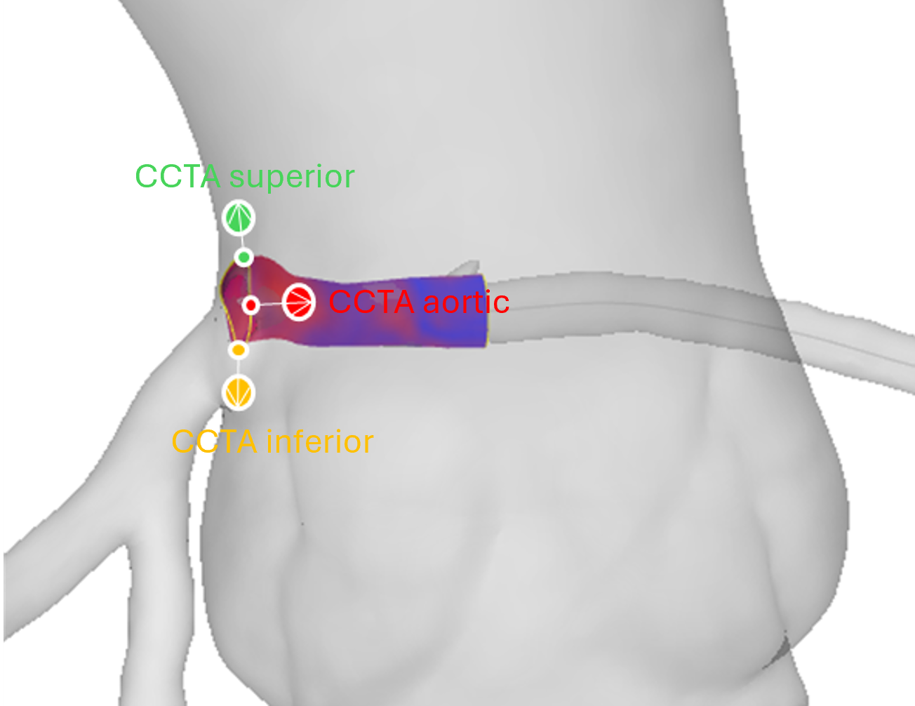
The reference contour is then best matched to these three points, all the leading points on the centerline are removed and the spacing is adjusted to match the z-spacing of the PyGeometry.

aligned_geometry, resampled_cl = mm.align_three_point(
    centerline=centerline,
    geometry_pair=rest,
    main_ref_pt=(12.2605, -201.3643, 1751.0554),
    counterclockwise_ref_pt=(11.7567, -202.1920, 1754.7975),
    clockwise_ref_pt=(15.6605, -202.1920, 1749.9655),
    write=True,
    watertight=False,
    interpolation_steps=0,
)

Preferred method: If you want to additionally use a pointcloud to finetune the three point alignment, by utilizing Hausdorff distances between the pointcloud and the geometry, multimodars.align_combined() can be used (see also CCTA tutorial on how to prepare the data to receive results['rca_points']):

aligned, resampled_cl = mm.align_combined(
    centerline,
    rest,
    (12.2605, -201.3643, 1751.0554),
    (11.7567, -202.1920, 1754.7975),
    (15.6605, -202.1920, 1749.9655),
    results["rca_points"],  # [(x, y, z), ...]
    angle_range_deg=10.0,
    write=True,
    watertight=True,
    output_dir="test",
)

5. Saving everything as .obj files

While every wrapper function allows to directly save the created geometries as .obj files (with optional interpolation), it is also possible to save any created geometry directly to an object file. The to_obj function can automatically detect the type of the object, and can be applied to PyGeometryPair, PyGeometry.

mm.to_obj(
    geometry,
    "output/dir",
    watertight=False,
    contour_types=[mm.PyContourType.Lumen, mm.PyContourType.Catheter],
    filename_prefix="aligned",
)

6. Utility functions to link to numpy

Converting objects to numpy — ``to_array``

multimodars.to_array() is a single dispatch-style function that converts any supported Py* object into numpy arrays. The return type depends on what is passed in:

stress_dia_arr, stress_sys_arr = mm.to_array(stress)   # PyGeometryPair → (dict, dict)
aligned_arr = mm.to_array(aligned)                     # PyGeometry → dict
centerline_arr = mm.to_array(cl_resampled)             # PyCenterline → ndarray
ostial_contour_arr = mm.to_array(rest.geom_a.frames[-1].lumen)  # PyContour → ndarray
frame_arr = mm.to_array(rest.geom_a.frames[0])         # PyFrame → dict
input_arr = mm.to_array(before_input_data)             # PyInputData → dict

The return value of multimodars.to_array() is one of the following, depending on the input type:

• multimodars.PyContour or multimodars.PyCenterline → np.ndarray of shape (N, 4), where each row is (frame_index, x, y, z).

• multimodars.PyFrame or multimodars.PyGeometry → dict[str, np.ndarray] with keys "lumen", "eem", "calcification", "sidebranch", "catheter", "wall", and "reference". Each value is a (M, 4) array of (frame_index, x, y, z) rows. The "reference" entry is (1, 4) when a reference point exists, or (0, 4) when absent.

• multimodars.PyGeometryPair → tuple[dict, dict], one dictionary per geometry (geom_a first, geom_b second), each in the same format as described for multimodars.PyGeometry above.

• multimodars.PyInputData → dict with the same layer keys as multimodars.PyGeometry, plus "diastole" (bool) and "label" (str). When records were supplied, a "records" key is added containing a (M, 4) object array of (frame, phase, measurement_1, measurement_2) rows.

Building a PyGeometry from numpy arrays — ``numpy_to_geometry``

When you already have aligned contour data as numpy arrays and want to construct a PyGeometry directly — for example after custom post-processing — use multimodars.numpy_to_geometry():

geometry = mm.numpy_to_geometry(
    lumen_arr=lumen_np,          # (N, 4) required: frame_index, x, y, z
    eem_arr=eem_np,              # (N, 4) optional
    catheter_arr=catheter_np,    # (N, 4) optional
    wall_arr=wall_np,            # (N, 4) optional
    reference_arr=ref_np,        # (1, 4) or (4,) optional
    label="my_geometry",
)

Rows with the same frame_index are grouped into a single PyFrame. The only required argument is lumen_arr; all other layers are optional and default to None (i.e. omitted from the resulting frames).

7. Class methods

PyContour

All transformation methods on PyContour return a new object and leave the original unchanged.

Centroid and geometry queries:

contour.compute_centroid()                            # recompute centroid in-place from points
pts = contour.points_as_tuples()                      # → list of (x, y, z) float tuples
(p1, p2), dist = contour.find_closest_opposite()      # nearest diametrically opposite pair
(p1, p2), dist = contour.find_farthest_points()       # widest pair of points
area          = contour.get_area()
elliptic_ratio = contour.get_elliptic_ratio()

• compute_centroid() — updates contour.centroid in-place from the current points list. Call this after manually editing points.

• points_as_tuples() — convenience accessor returning [(x, y, z), ...] without the frame-index column; useful for plotting or passing to third-party mesh libraries.

• find_closest_opposite() — finds the pair of points separated by the smallest diameter (minimum Feret diameter), returned as ((p1, p2), distance).

• find_farthest_points() — finds the pair of points separated by the largest Euclidean distance (maximum Feret diameter).

• get_area() and get_elliptic_ratio() — CAVE: both methods use the coordinate values directly; if contours are in pixel units the results are meaningless. Always provide coordinates in mm.

Transformations and point ordering:

contour_rot    = contour.rotate(20.0)                  # rotate 20° around the centroid
contour_trsl   = contour_rot.translate(0.0, 1.0, 2.0)  # translate by (dx, dy, dz) in mm
contour_sorted = contour.sort_contour_points()          # reorder points clockwise

• rotate() — rotates the contour in the xy-plane by angle_deg degrees around its centroid. Returns a new PyContour.

• translate() — shifts every point by (dx, dy, dz) mm. Returns a new PyContour.

• sort_contour_points() — reorders points into a consistent clockwise winding order. Useful before area calculations or mesh construction.

To write a modified contour back into a geometry, construct a new PyFrame and call replace_frame():

old_frame = geometry.frames[2]
new_lumen = old_frame.lumen.rotate(20.0)
new_frame = mm.PyFrame(
    id=old_frame.id,
    centroid=old_frame.centroid,
    lumen=new_lumen,
    extras=old_frame.extras,
    reference_point=old_frame.reference_point,
)
geometry = geometry.replace_frame(2, new_frame)

PyFrame

PyFrame aggregates the lumen contour, optional extra layers, and the reference point for a single imaging position. Its transformation methods mirror those of PyContour and all return a new frame:

frame_rot    = frame.rotate(20.0)                # rotate all contours in the frame
frame_trsl   = frame.translate(0.0, 1.0, 2.0)   # translate all contours by (dx, dy, dz)
frame_sorted = frame.sort_frame_points()          # reorder all contour points clockwise

• rotate() — applies the same rotation to every contour in the frame.

• translate() — shifts every contour by the given offset.

• sort_frame_points() — calls sort_contour_points() on all contours in the frame.

PyGeometry / PyGeometryPair

PyGeometry exposes methods for querying individual frames, traversing contour layers, and transforming or resampling a full pullback geometry.

Frame access and contour retrieval:

frame    = geometry.get_frame_at_index(5)              # frame by sequential index (0-based)
frame    = geometry.get_frame_at_z(12.5)               # frame whose z is closest to 12.5 mm
contours = geometry.get_lumen_contours()               # list of all lumen PyContour objects
contours = geometry.get_contours_by_type("Wall")       # any layer by its kind string
geometry = geometry.replace_frame(2, new_frame)        # returns a new PyGeometry

• get_frame_at_index() — zero-based positional look-up along the pullback axis.

• get_frame_at_z() — spatial look-up; returns the frame whose centroid z-coordinate is nearest to the requested value.

• get_lumen_contours() — equivalent to get_contours_by_type("Lumen") but slightly faster.

• get_contours_by_type() — accepts any kind string (e.g. "Eem", "Wall", "Catheter").

• replace_frame() — immutable update; returns a new PyGeometry with frame at index replaced.

Geometry-level transformations:

geom_smooth  = geometry.smooth_frames()               # 3-point moving average on all contours
geom_rot     = geometry.rotate(20.0)                  # rotate all frames
geom_trsl    = geom_rot.translate(0.0, 1.0, 2.0)     # translate all frames by (dx, dy, dz)
geom_ds      = geometry.downsample(100)               # resample every contour to 100 points
geom_sorted  = geometry.sort_frame_points()           # reorder contour points in all frames
geom_centred = geometry.center_to_contour(mm.PyContourType.Catheter)

• smooth_frames() — applies a 3-point moving-average filter to each contour across the frame sequence, reducing discretisation artefacts.

• downsample() — resamples every contour to exactly n_points evenly-spaced points. Useful for normalising contour resolution before comparison.

• sort_frame_points() — propagates sort_frame_points() across all frames.

• center_to_contour() — recentres the coordinate system so that the centroid of the chosen contour type (e.g. PyContourType.Catheter) lies at the origin for every frame.

Summaries and measurements:

get_summary() returns a (mla, max_stenosis_pct, stenosis_len_mm) tuple for a single PyGeometry. On a PyGeometryPair it returns a nested tuple plus a per-frame deformation table that can be cast directly to numpy:

mla, stenosis_pct, stenosis_len = geometry.get_summary()       # PyGeometry

(summary_a, summary_b), deformation = geometries.get_summary() # PyGeometryPair
# summary_a / summary_b: (mla, max_stenosis_pct, stenosis_len_mm)
deform_array = np.array(deformation)  # shape (N, 6): id, area_dia, ellip_dia, area_sys, ellip_sys, z

Returns:

Geometry "Diastole":
MLA [mm²]: 5.57
Max. stenosis [%]: 58
Stenosis length [mm]: 2.99

Geometry "Systole":
MLA [mm²]: 4.71
Max. stenosis [%]: 69
Stenosis length [mm]: 11.20

+----+----------+-----------+----------+-----------+-------+
| id | area_dia | ellip_dia | area_sys | ellip_sys |   z   |
+----+----------+-----------+----------+-----------+-------+
| 0  | 12.20    | 1.23      | 15.14    | 1.03      | 0.75  |
| 1  | 12.68    | 1.20      | 14.99    | 1.04      | 1.49  |
| 2  | 13.09    | 1.16      | 14.85    | 1.05      | 2.24  |
| 3  | 13.24    | 1.13      | 14.51    | 1.04      | 2.99  |
| 4  | 13.26    | 1.11      | 13.48    | 1.03      | 3.73  |
| 5  | 13.22    | 1.12      | 11.78    | 1.06      | 4.48  |
| 6  | 13.07    | 1.11      | 9.50     | 1.11      | 5.23  |
| 7  | 12.70    | 1.10      | 7.86     | 1.13      | 5.97  |
| 8  | 12.46    | 1.10      | 6.87     | 1.18      | 6.72  |
| 9  | 12.37    | 1.09      | 6.62     | 1.18      | 7.46  |
| 10 | 12.28    | 1.08      | 6.28     | 1.21      | 8.21  |
| 11 | 12.04    | 1.09      | 5.91     | 1.26      | 8.96  |
| 12 | 11.77    | 1.12      | 5.56     | 1.32      | 9.70  |
| 13 | 11.06    | 1.14      | 5.58     | 1.37      | 10.45 |
| 14 | 10.09    | 1.12      | 5.96     | 1.48      | 11.20 |
| 15 | 8.93     | 1.11      | 6.31     | 1.59      | 11.94 |
| 16 | 7.85     | 1.14      | 6.35     | 1.87      | 12.69 |
| 17 | 6.80     | 1.16      | 5.81     | 2.27      | 13.44 |
| 18 | 5.99     | 1.30      | 5.29     | 2.76      | 14.18 |
| 19 | 5.57     | 1.55      | 5.25     | 2.97      | 14.93 |
| 20 | 5.86     | 1.78      | 5.42     | 2.88      | 15.68 |
| 21 | 6.04     | 1.76      | 5.45     | 2.79      | 16.42 |
| 22 | 6.55     | 1.53      | 5.02     | 2.66      | 17.17 |
| 23 | 7.22     | 1.43      | 4.71     | 2.56      | 17.92 |
+----+----------+-----------+----------+-----------+-------+